Decision makers are always looking for ways to understand the effects of their actions. Managers generally assume that if they find a correlation between two items it means they understand the relationship between two variables; however, as was stated in a previous blog article, Beware of Correlations, correlations may not tell the whole story, and, furthermore, they can only tell the story between two variables. Regression allows us to understand more involved relationships between variables and an outcome variable.

Regression attempts to predict a response variable from 1 or more independent variables, i.e. we take some data and try and predict something based on it. Investigating the effect of the predictor variables on a response variable is known as exploring the causal effect. For example, you might want to predict sales from a number of variables such as annual compensation of executives based on years of experience, age, and years of education.

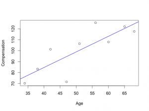
The best way to think about regression would be image a series of data points, such as compensation and age. Lets say we collect compensation data by interviewing executives and managers. The data collected is represented in the following chart. Added to the chart is a line that we drew that represents the trend of the data, and a good prediction lines, such that if you pick an age and plot it on the line, that would be the best estimate of their compensation level. Thus, a person 55 years of age would be expected to have a salary compensation of about 106,000.

While there are many types of regression, this article demonstrates the two most common types of regression, simple linear regression and multiple linear regression. They are essentially the same procedure of examining the effect on a single predictor variable(y), with the only difference being that simple linear regression contains one predictor variable (single x variable), and multiple linear regression contains many predictor variables (multiple x variables).

Thus, a regression equation looks like the following:

The betas, in the equation are called coefficients. Each independent variable (x) has a coefficient attached to it. It is the estimate that when multiplied by x gives the best representation of the change in y. The Beta “zero”, the first coefficient, is called the intercept, and represents the value if the x variable was 0. This itself may not make sense but we will address that in a future article. However, in the example above, if one the regression was run for the data above, the following equation would be obtained.

It means that to predict the compensation level, take a persons age, multiply it by 1.4, then add 27.4. Therefore, this model is a starting point to predict the value of compensation based on age.

There are a number of assumptions that are required for regression, which will be addressed in the next article.